kitaev-mf: Majorana mean-field theory
What survives of the exactly solvable Kitaev spin liquid when a magnetic field, a defect, or additional interactions prevent an exact solution? The open-source project kitaev-mf approaches this question through a self-consistent Majorana mean-field approximation, combining analytical structure with reproducible numerical calculations.
The first stage concentrates on the ferromagnetic Kitaev honeycomb model in a magnetic field along \([111]\): establishing the algebra, constructing the Gaussian mean-field states, and determining when numerical solvers can be trusted. From there, the program turns to low-energy excitations, vortices, dynamical response, and models outside the integrable limit. The distinction between a converged calculation and a controlled physical approximation guides the work throughout.
From spins to a Majorana mean-field state
The honeycomb Kitaev interaction couples a different spin component on each bond. With Pauli operators \(\sigma_i^\gamma\) and a choice of exchange-sign convention, the spin Hamiltonian can be written as
At zero field, the Kitaev representation introduces four Majorana operators \(c_i^\mu\) per site, obeying \(\{c_i^\mu,c_j^\nu\}=2\delta_{ij}\delta^{\mu\nu}\). The representation enlarges the Hilbert space: local physical-state projection is essential. In the integrable model, one can choose a static \(\mathbb{Z}_2\) gauge sector and solve a quadratic Hamiltonian for the remaining matter Majoranas. Generic magnetic fields couple the matter and gauge degrees of freedom, so the same exact reduction no longer applies.
The mean-field approximation restricts the state to a quasifree (Gaussian) fermionic family. Within this family, Wick's theorem expresses higher even correlations in terms of two-point functions. This is a property of the chosen states, not an operator identity for the original interacting Hamiltonian. The calculation is parametrized by directed-bond covariances \(U_{ij}^{\mu\nu}\), on-site covariances \(V_i^{\mu\nu}\), and multipliers \(\lambda_i^\gamma\) for the local constraints. In the conventions of the project's labbook,
The superscript \(\mathrm G\) indicates a Gaussian state. Bond orientation, the sign convention of the spin–Majorana representation, and the normalization of exchange couplings must remain consistent when comparing calculations.
Self-consistency as a nonlinear spectral problem
Collect the independent mean-field variables into \(X=(U,V,\lambda)\). They determine a quadratic Hamiltonian \(H_{\mathrm{MF}}[X]\), whose occupied single-particle states produce new covariances. Updating the constraints alongside these covariances defines a nonlinear map
For a gapped zero-temperature Bloch Hamiltonian, the underlying covariance update can be expressed using its occupied spectral projector,
At zero modes or finite-size level crossings, occupations and physical parity require additional care. The simplest solver repeats \(X_{n+1}=\Phi(X_n)\) (Picard iteration). Damping instead uses \(X_{n+1}=X_n+\alpha R(X_n)\), where \(0<\alpha\le1\). Local linear convergence is governed by the derivative of the iteration map; neither damping nor convergence is guaranteed throughout the full parameter space.
The code also investigates Anderson acceleration / DIIS, Broyden updates, and Jacobian-free Newton–Krylov methods. DIIS combines a history of residuals; Broyden approximates the inverse response of \(R\); limited-memory variants avoid storing a dense Jacobian. In large real-space problems, evaluating \(\Phi\) itself is expensive, motivating real skew-symmetric linear algebra and matrix-sign purification of Gaussian covariances. Near a vanishing spectral gap, these spectral algorithms need conditioning and zero-mode safeguards.
Finding \(R(X_*)\simeq0\) does not prove that \(X_*\) is the global minimum of the mean-field energy, that it satisfies every physical constraint, or that the Gaussian state accurately represents the interacting spin ground state. Multiple self-consistent solutions can coexist. Their energies, local stability, admissibility, and dependence on initial conditions must be examined separately.
What can numerical benchmarks establish?
Three logically distinct questions must be tested.
Is the calculation algebraically and numerically consistent? The CAR normalization, antisymmetry of Majorana covariances, Hermiticity of the effective one-particle Hamiltonian, spectral sum rules, positivity constraints, and gauge/KKT residuals should survive changes in lattice size and solver. A small fixed-point residual alone is insufficient.
Does the approximation reproduce a result known independently? In the zero-field, flux-free isotropic Kitaev limit, the matter dispersion is controlled by \(f(\mathbf k)=1+e^{2\pi i k_1}+e^{2\pi i k_2}\). An exact integral provides a particularly useful bond-covariance benchmark:
In the labbook's ferromagnetic, flux-free gauge convention, \(U_b^{00}=-\bar U\). Other exact checks include band folding, the anisotropic one-dimensional zigzag limit, and isolated-bond dimers.
The midpoint rule approximates the integral above on an N × N grid, with ka = (na + 1/2)/N. It is a numerical approximation to a known exact-limit quantity, not a mean-field solver benchmark.
| N | Midpoint Ū | Absolute difference |
|---|---|---|
| 8 | 0.5248951470 | 2.94 × 10⁻⁵ |
| 16 | 0.5248532248 | 1.25 × 10⁻⁵ |
| 32 | 0.5248651506 | 5.95 × 10⁻⁷ |
| 64 | 0.5248656070 | 1.39 × 10⁻⁷ |
| 128 | 0.5248657324 | 1.34 × 10⁻⁸ |
Reference Ū = 0.5248657458506. The error need not decrease monotonically with N; the integral has zeros where |f| is not smooth. The static table remains visible without JavaScript.
These constrain the implementation in special regimes; they do not establish the accuracy of an arbitrary finite-field mean-field solution.
Jx = Jy = J; vary 0 ≤ Jz ≤ 2J. The static view shows Jz = J. Colors share the fixed range r = 0–4.
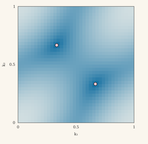
Exact zero-field flux-free structure factor, not the finite-field mean-field excitation energy.
Is a physical prediction robust? Compare independent initial states and solver families, scan system size and boundary conditions, inspect competing stationary branches, and check observables against perturbation theory or exact diagonalization where possible. Spin-correlation sum rules and physically projected flux/parity sectors matter as much as convergence speed. An approximation without a uniform error bound remains uncontrolled even after excellent numerical validation.
The project's Living Lab Book develops these checks in detail, from covariance positivity and spectral projectors to fixed-point basins and real-space purification. Its numerical tables are regime-specific evidence, not universal solver rankings or proofs of physical accuracy.
Physics beyond the integrable limit
Exact perturbation theory versus mean field. A weak magnetic field generates an effective chiral interaction at third order, schematically of order \(h_xh_yh_z\). In exact spin perturbation theory, intermediate states involve changed flux sectors and the physical Hilbert-space projection. In a Gaussian mean-field calculation, the intermediate excitations and self-consistent responses differ. Comparing coefficients therefore requires matching conventions, spectral thresholds, and the relevant resolvents; replacing a denominator by a single flux-gap estimate is not an exact derivation.
Low-energy physics of the Kitaev spin liquid. The zero-field matter sector has Dirac points. Weak fields, vortices, and boundaries introduce questions about induced gaps, bound modes, spin correlations, and their observable signatures. The project's longer-term dynamical program will compare exact gauge-quench spin correlators with their mean-field counterparts, including the tunneling response associated with vortex-bound Majorana modes.
Other phases and solvable limits. The anisotropic chains and decoupled dimers supply exact benchmark corners. High-field polarization supplies a different asymptotic reference, but a generic finite-field honeycomb model is not made exactly solvable by being close to that limit. Extending the method to other couplings and phases requires separate analysis of the relevant low-energy degrees of freedom and the validity of the Gaussian ansatz; a converged solution by itself cannot classify a phase.
Numerical methods as a research question. Beyond computing a phase diagram, the project asks which fixed-point algorithms remain reliable near competing phases, small gaps, vortices, disorder, or large real-space systems. One must separate iteration count from wall-clock cost, local convergence from basin reliability, and solver failure from a genuine physical instability.
Further notes in this series
The topics below are planned as separate, self-contained articles. Links will be added when each article is written, checked, and published; no empty note pages are exposed.
| Theme | Planned article |
|---|---|
| Exact reference | Exact Kitaev spectra, physical parity, and perturbative resolvents |
| Low-energy theory | Dirac matter, field-induced masses, and vortex excitations |
| Other regimes | Anisotropic chains, dimers, and polarized limits |
| Validation | When a converged Majorana mean field can be trusted |
| Numerics I | Fixed-point iteration and the map \(\Phi\) |
| Numerics II | DIIS, Anderson, Broyden, and Newton–Krylov methods |
| Numerics III | Matrix-sign purification and large real-space lattices |
| Dynamics | Spin correlations, gauge quenches, and tunneling spectroscopy |
Further reading: project source code · Living Lab Book (PDF) · project roadmap · exact-perturbation research notes.